How to Hide Columns in Excel

Microsoft Excel is an incredibly versatile spreadsheet program used by millions of people worldwide. One frequently used feature of Excel is the ability to hide columns for a variety of reasons. Whether you’re trying to focus on specific data or simply decluttering a large spreadsheet, hiding columns can be an effective way to simplify your view. In this blog post, you’ll discover a straightforward way to hide columns in Excel, allowing you to customize your spreadsheet to your liking.
Why Hide Columns in Excel?
Hiding columns in Excel can make your data easier to read. This can be especially important when you have a larger spreadsheet, making it difficult to read and understand. Additionally, hiding columns can help you focus on the necessary data, so you can complete your work more efficiently.
Steps to Hide Columns in Excel
Step 1: Select the Column
To hide a column in Excel, you’ll first need to find the column you want to hide. Select the column by clicking on the letter at the top of the column.
Step 2: Right-Click on the Column Header
Once you have selected the column, right-click on the column header. A drop-down menu will appear.
Step 3: Select “Hide” from the Drop-Down Menu
From the drop-down menu, select the “Hide” option. The selected column will disappear from view.
Unhiding Columns in Excel
Step 1: Highlight the Columns on Either Side of the Hidden Column
To unhide a column in Excel, you’ll need to highlight the columns on either side of the hidden column. You do this by clicking on the letter at the top of the column to the left, then dragging the cursor across to the right and highlighting each column until you reach the column to the right of the hidden column.
Step 2: Right-Click on the Column Header
Once you’ve highlighted the columns on either side of the hidden column, right-click on the column header. A drop-down menu will appear.
Step 3: Select “Unhide” from the Drop-Down Menu
From the drop-down menu, select the “Unhide” option. The hidden column should now be visible.
By following these simple steps, hiding and unhiding columns in Excel can be a breeze. This is just one of the many ways Excel can help simplify your life.
Keeping Hidden Columns Safe
Hiding columns in Excel is a great way to declutter your spreadsheet and make it more readable. However, it is easy to forget which columns are hidden when you reopen your Excel document. To keep your hidden columns safe, you can protect your Excel worksheet by following these simple steps:
- Go to the “Review” tab in the Excel ribbon
- Select “Protect Sheet”
- Enter a password to protect the sheet and check the “Hidden” checkbox under the “Cells” section
- Select “OK”
This will ensure that only those with the password can unhide the columns and protects your data from being accidentally modified.
Alternate Method to Hide Columns in Excel
In addition to the previously mentioned method, there is another way to hide columns in Excel:
- Select the columns you want to hide
- Right-click on the selection and choose “Hide”
- Press the “Ctrl” and “0” keys together to hide the selected columns at once
This method combines the first two steps from the earlier method and can be a faster way to hide multiple columns.
Using the “Format Only Cells That Contain” Feature to Hide Columns
Excel has a feature called “Format Only Cells That Contain” that can also be used to hide columns. Here’s how:
- Select the columns you want to hide
- Go to the “Home” tab in the Excel ribbon and click “Conditional Formatting”
- Select “New Rule…”
- In the “New Formatting Rule” dialog, select “Use a formula to determine which cells to format”
- In the formula field, enter “=COLUMN()=X”, where “X” is the column number you want to hide
- Click “Format” and select the “Font” tab
- Check the “Color” checkbox and select a color that matches your background color
- Click “OK” to close the “Font” dialog, then click “OK” again to close the “New Formatting Rule” dialog
By following these steps, the column(s) you want to hide will now appear invisible as they match the background color of the spreadsheet. However, be cautious as the hidden columns will still be visible if the background color is changed.
Excel can be a powerful and efficient tool, but it can be overwhelming without a basic understanding of how it works. Hiding columns is an easy way to make your data more readable and streamlined. Whether it is to eliminate clutter or protect the data, hiding columns in Excel can be an excellent solution to reveal only the crucial information. The ability to hide specific columns in Excel, amongst other features, is what has made it the go-to application for data management of all kinds, making it a valuable skill to learn.
FAQs
Here are some frequently asked questions about hiding columns in Excel:
Can I hide multiple columns at once in Excel?
Yes! You can select multiple columns and hide them simultaneously by right-clicking the selection and choosing “Hide.”
Can hidden columns still be included in formulas and calculations?
Yes. Hidden columns can still be included in formulas and calculations. However, it is essential to be careful while comparing data side-by-side with hidden columns as they are still present in the entire dataset.
How can I unhide columns in Excel?
To unhide columns in Excel, you need to highlight the columns on either side of the hidden column, right-click on the column header, and select “Unhide” from the dropdown menu. You can also select the entire worksheet, click “Format,” then “Hide & Unhide,” and choose “Unhide Columns.”
Can I password protect my hidden columns?
Yes. You can protect your Excel worksheet by password-protecting the sheet and checking the “Hidden” checkbox under the “Cells” section. Doing so will ensure that only those with the password can unhide the columns.
How can I make sure I don’t forget which columns I’ve hidden?
If you’re worried you might forget which columns you’ve hidden, you can use the “Custom Views” feature in Excel. Here’s how:
- Go to “View” in the Excel ribbon and select “Custom Views”
- Select “Add”
- Type in a name for this view, and check “Hidden Rows, Columns, and Filter Settings”
- Click “OK”
This will save your current view of the spreadsheet, with hidden columns included. The next time you open the spreadsheet, you can go back to the “Custom Views” and select the saved view to get the previous settings back.