How to Hide Cells in Excel

Microsoft Excel is a powerful tool that assists you in organizing, manipulating, and analyzing data efficiently. It includes numerous features that make your work more manageable and less time-consuming. One of Excel’s many features is the ability to hide cells, which can be beneficial in several ways, such as protecting sensitive information or hiding unnecessary data. This blog post will explore how to hide cells in Excel, providing you with a quick and direct answer to this question.
Introduction
If you’ve ever wanted to hide cells in Excel, you’re in the right place. Hiding cells can be beneficial for several reasons: it can prevent other people from seeing sensitive information, organize your spreadsheet by hiding excess data, or just declutter your view. Whatever the reason, Excel provides an easy way to hide cells, and this article will show you how.
Step by Step Guide
Step 1: Select the cells you want to hide
Before you can hide the cells, you need to select them. If you want to hide an entire column or row, click the row number or column letter at the top of the sheet. If you want to hide specific cells, click and drag your mouse over them to select them. Alternatively, if the cells you want to hide are contiguous, click on the first cell, hold down the shift key, and click on the last cell to select them all at once.
Step 2: Right-click and select “Hide”
Once you have selected the cells you want to hide, right-click on them and select “Hide” from the context menu. If you have selected an entire column or row, the option to hide them will be directly in the context menu. If you have selected specific cells, you will need to click “Hide” under the “Hide & Unhide” submenu.
Step 3: Verify that the cells are hidden
After hiding the cells, you might want to verify that they have been hidden correctly. You can tell by looking for gaps in your column or row labels. If you’ve hidden an entire column and there are no other greyed-out columns in your sheet, you’ll notice that the column is now missing. If you’ve hidden specific cells, you won’t see them, but if you select the cells immediately before and after the hidden cells, you’ll see that there is a gap.
Show Hidden Cells
Step 1: Select the range that contains the hidden cells
If you need to view hidden cells again, you’ll need to unhide them. To do so, select the range that contains the hidden cells. If a column or row is hidden, select the entire row or column by clicking on its label. If specific cells are hidden, select the cells surrounding the hidden cells.
Step 2: Right-click and select “Unhide”
Next, right-click on the selected range and choose “Unhide” from the context menu. If you hid an entire row or column, Excel will unhide the entire row or column. If you hid specific cells, Excel will unhide those cells without affecting any other cells in the range.
Step 3: Verify that the cells are unhidden
If you’ve unhidden the cells correctly, you’ll see the previously hidden cells again displayed in your spreadsheet.
Excel’s ability to hide cells can make organizing data and protecting sensitive information easier. Now that you know how to hide and unhide cells in Excel, you can manipulate and organize your data even more confidently and efficiently.
You Can Hide Formulas Too
Did you know that you can hide formulas in your Excel sheet to prevent others from accidentally editing them? This feature will ensure that any sensitive or important data that you have calculated in formulas is protected. To hide formulas, select the cell with the formula you want to hide, and then press Ctrl + 1 or right-click on the cell and select “Format Cells” from the context menu. In the “Format Cells” dialog box, click on the “Protection” tab and check the box next to “Hidden.” Next, click “OK” to close the dialog box. Now, anyone who tries to edit the cell will see the formula bar and know that there is a calculated formula in that cell, but they won’t be able to see the actual formula.
How to Protect Hidden Cells
Hiding cells can be a great way to keep your data clean and prevent others from accidentally editing sensitive information. But what if someone else who has access to your Excel sheet wants to unhide a cell that you’ve hidden? Fortunately, there’s a simple solution: protect your hidden cells. You can protect your hidden cells by going to the “Review” tab in Excel’s ribbon and selecting “Protect Sheet.” In the “Protect Sheet” dialog box, check the box next to “Hidden” to ensure that all hidden cells are protected. Then set a password to prevent anyone from accidentally unchecking the “Hidden” box, and click “OK.” Now your hidden cells are fully protected, and you can still view them when you need to.
Whether you’re working with sensitive data or you just want to declutter your view, hiding cells in Excel can be a helpful tool. With these simple steps, you can make sure that your data is organized and protected from unauthorized changes.
FAQ
Here are some common questions related to hiding cells in Excel.
Can I hide multiple rows or columns at once?
Yes, you can hide multiple rows or columns at once by selecting the entire row or column you want to hide, right-clicking, and selecting “Hide.” Alternatively, you can also select multiple rows or columns by clicking and dragging your mouse over the row or column labels at the top of the sheet and then right-click and select “Hide.”
How can I tell if a cell is hidden?
If you’ve hidden a cell in Excel, you can tell that it is hidden by looking for a gap where the cell should be. If you want to verify that the cell is hidden, click on the cell immediately before or after the hidden cell, and you’ll see that there is a gap. You can also check whether a row or column is hidden by looking at the row or column labels; a hidden row or column will have a gap in the numbering or letters.
How can I hide cells without changing the formatting?
When you hide cells in Excel, the formatting of the hidden cells will be preserved. However, if you want to hide the cells without changing the formatting, you can do so by adjusting the column width or row height to 0. This will effectively hide the cells, and their formatting will remain intact. To do so, select the column or row you want to hide, right-click, and select “Column Width” or “Row Height.” Enter “0” in the “Column Width” or “Row Height” box, and click “OK.”
How do I unhide multiple rows or columns at once?
If you want to unhide multiple rows or columns at once, select the rows or columns immediately before and after the hidden rows or columns, right-click on the selection, and select “Unhide.” Excel will unhide any hidden rows or columns in the selected range.
Can I print a sheet with hidden cells?
Yes, you can print an Excel sheet that includes hidden cells, but the hidden cells will still be hidden in the printed version. To print a sheet with hidden cells, go to the “File” tab, select “Print,” and click on “Print Options.” Under “Sheet Options,” check the box that says “Print,” and then click “OK” to print the sheet with the hidden cells.